Sales pipeline forecasting methods: Stage vs Cycle in 2026

Choosing between different sales pipeline forecasting methods often determines whether your revenue projection reflects real incoming cash or wishful executive thinking. Sales leaders frequently find themselves caught between two opposing schools of thought: should you calculate pipeline value based on the milestone stage an opportunity has reached, or should you forecast close dates based on the calendar time that has elapsed since the lead entered your funnel? Choose stage probability forecasting if your team runs structured, milestone-driven B2B deals with verifiable buyer commitments; choose sales cycle length forecasting if your business operates on high-volume, standardized velocity where time elapsed is the strongest predictor of deal mortality. This guide compares both methods across baseline accuracy, stale deal treatment, CRM data maturity requirements, sales rep adoption, and forecast volatility.

Sales pipeline forecasting methods: Stage probability vs sales cycle length at a glance

Stage probability forecasting (often called weighted pipeline forecasting) calculates expected revenue by multiplying the nominal value of each open deal by a fixed win probability assigned to its current pipeline stage. In contrast, sales cycle length forecasting calculates when deals will close by projecting historical average conversion time onto active opportunities, treating time elapsed as the primary determinant of deal viability. The core operational difference lies in what each model trusts most: stage probability trusts milestones, while sales cycle forecasting trusts the calendar clock.

Criterion	Stage Probability Forecasting	Sales Cycle Length Forecasting	Better Pick
Core Calculation Driver	Deal position in defined pipeline stages	Historical days elapsed from deal creation	Context dependent
Formula Mechanism	Deal Value ($) × Stage Win Probability (%)	Opportunity Creation Date + Historical Cycle Days	Stage Probability
Treatment of Stale Deals	Treats a 90-day-old proposal the same as a 2-day-old proposal unless manually adjusted	Flags or discounts deals exceeding normal velocity benchmarks	Sales Cycle Length
Sensitivity to Rep Bias	High; reps inflate stages due to optimistic sentiment	Low; relies on objective calendar timestamps	Sales Cycle Length
CRM Data History Needed	Low; requires 30 to 60 days of conversion ratios	High; requires 6 to 12 months of clean cycle duration logs	Stage Probability
Suitability for Enterprise B2B	Excellent; matches complex milestone procurement	Poor; enterprise deals rarely follow linear timelines	Stage Probability
Suitability for High-Volume SMB	Moderate; heavy administration overhead	Excellent; leverages law of large numbers and velocity	Sales Cycle Length
Volatility Near Quarter-End	High if large deals slip stages abruptly	Moderate; slips are identified weeks in advance	Sales Cycle Length
Ease of Team Implementation	Immediate; native to almost all CRM platforms	Requires dedicated velocity reports or custom date logic	Stage Probability

For organizations evaluating modern sales forecasting software, understanding the mechanical differences between these two methodologies is essential before configuring CRM pipeline rules.

What are stage probability and sales cycle length forecasting?

Before comparing their mechanics, revenue leaders must understand the foundational problem each method was engineered to solve within daily pipeline management. Neither approach was created to provide a perfect crystal ball, but rather to establish a repeatable mathematical baseline for revenue predictability.

Opportunity stage probability forecasting explained

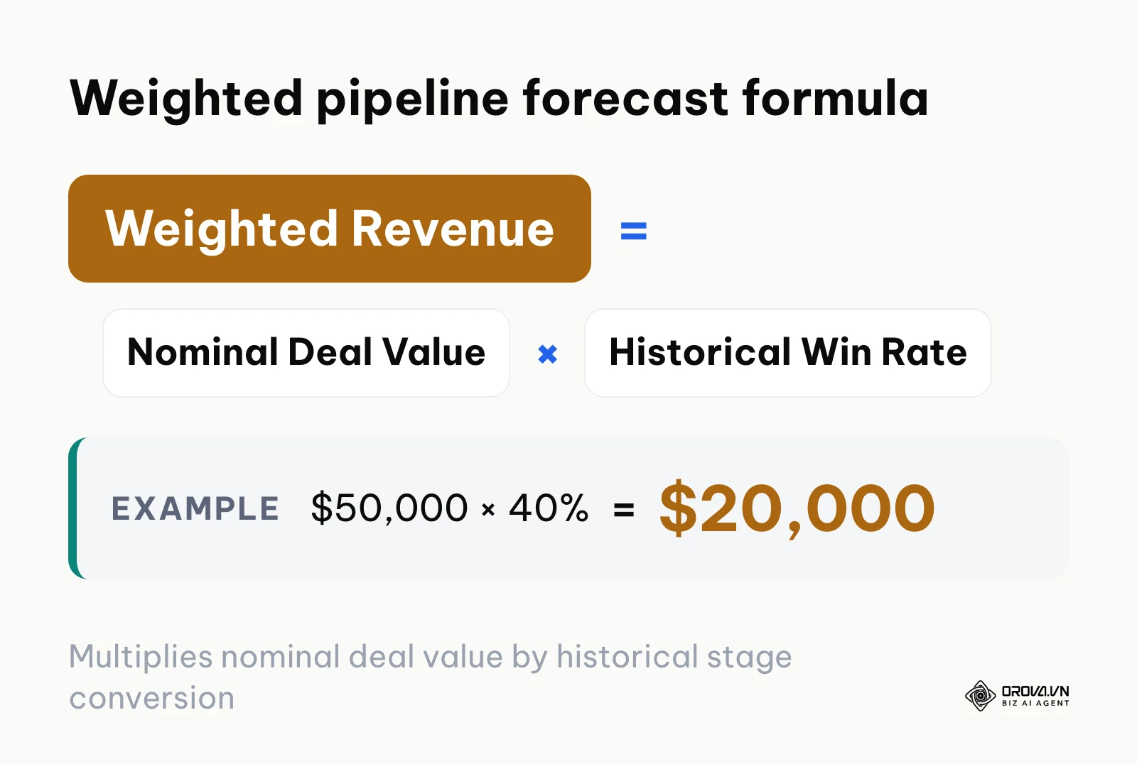
Opportunity stage probability forecasting is a milestone-based quantitative projection method that assigns an incremental win likelihood to each sequential phase of a sales process. As an opportunity moves from initial discovery to formal demonstration, technical evaluation, commercial proposal, and contract negotiation, the assigned probability increases from perhaps 10% to 80%. Multiplying nominal deal value by these fixed stage percentages generates a "weighted pipeline" value designed to reflect the mathematical expected value of the current pipeline.

Sales cycle length forecasting explained

Sales cycle length forecasting is a time-series quantitative projection method that estimates close dates by analyzing the historical average duration required for similar opportunities to move from creation to closed-won status. Instead of trusting where the salesperson claims the deal stands emotionally, this method projects expected revenue into specific fiscal periods based strictly on the age of the deal relative to historical velocity benchmarks. It operates on the core operational principle that deal momentum degrades predictably over time.

Baseline projection accuracy: Stage probability vs sales cycle length

Baseline projection accuracy depends entirely on whether deal value or deal velocity fluctuates more within your specific sales motion. According to the Sales Forecasting: Driving Predictable Revenue Growth report published by Gartner in 2024, over 67% of B2B revenue organizations struggle with forecast variance exceeding 10% because their pipeline milestones rely on subjective rep sentiment rather than verifiable buyer commitments.

When opportunity stage probability operates in an organization with rigorously enforced stage definitions, its baseline accuracy is remarkably consistent. For example, if a team has closed 100 enterprise software deals over two years and consistently converts 40% of deals that reach formal proposal review, applying a 40% weighting to five active proposals totaling 500,000 dollars reliably projects 200,000 dollars in gross revenue. The weakness of this approach is that it assumes every deal in that stage has an identical chance of closing, completely ignoring whether a prospect has been actively reading emails or ignoring follow-ups for six weeks.

Sales cycle length forecasting delivers superior accuracy when dealing with high-velocity transactional sales where deal values are relatively uniform. If an inside sales team closes inbound SaaS subscriptions with an average deal size of 6,000 dollars and an average sales cycle of 32 days, calculating close probability based on deal age produces an exceptionally tight forecast. If a deal reaches Day 45 without closing, the historical model correctly identifies that its true win probability has collapsed to near zero, regardless of what the rep hopes will happen.

Worked example:

• Context: A mid-market logistics software company with 8 account executives managing 60-day average sales cycles.
• Steps taken: The sales operations manager pulled historical CRM data for 140 past opportunities, calculated conversion rates for each stage, and compared the resulting stage-weighted forecast against an age-based velocity projection for the upcoming quarter.
• Snag encountered & fix: The stage-weighted model projected 850,000 dollars in closed business, while the cycle-length model projected only 580,000 dollars. Upon auditing individual records, the manager discovered three massive enterprise proposals worth 320,000 dollars that had been sitting in the proposal stage for over 110 days without customer activity. The manager applied an aging discount to the stage model.
• Visible operational result: The team finished the quarter at 610,000 dollars, aligning closely with the cycle-adjusted baseline while exposing the unaddressed stall in enterprise pipeline progression.

Stage probability provides better baseline accuracy for customized B2B sales with variable contract values, while sales cycle length provides superior baseline accuracy for standardized transactional sales motions.

Handling stale deals and aging decay: Stage probability vs sales cycle length

The single largest blind spot in conventional pipeline management is the treatment of stale deals, also known as pipeline debt. A deal that has lingered in the proposal stage for 90 days cannot mathematically retain the same 50% win probability as a deal that entered that stage yesterday. Research published in the Harvard Business Review report Why Sales Forecasts Always Miss in 2023 revealed that opportunities lingering in a single sales stage longer than 1.5 times the company average experience a 62% decline in ultimate win rate, regardless of the rep's reported confidence.

Standard stage probability forecasting completely ignores this dynamic. If an opportunity worth 100,000 dollars sits at the contract stage (75% probability) for six months, the traditional weighted formula continues to credit the forecast with 75,000 dollars in expected revenue month after month. This creates a phantom pipeline that deceives finance teams, masks lead generation shortfalls, and leads to dramatic quarter-end revenue misses.

Sales cycle length forecasting inherently penalizes deal stagnation. Because the model relies on calendar timestamps, an opportunity that exceeds historical duration thresholds automatically falls out of near-term forecast windows. To reconcile this difference, advanced RevOps teams implement an aging decay formula within their milestone forecasting:

$$\text{Adjusted Value} = \text{Nominal Value} \times \text{Base Win Probability} \times (1 - \text{Aging Decay Penalty})$$

Where the aging decay penalty is defined by the formula:

$$\text{Aging Decay Penalty} = \begin{cases} 0\% & \text{if Stage Dwell Time} \le \text{Benchmark Dwell Time} \\ 50\% & \text{if Benchmark} < \text{Dwell Time} \le 2.25 \times \text{Benchmark} \\ 60\% \text{ to } 80\% & \text{if Dwell Time} > 2.25 \times \text{Benchmark} \end{cases}$$

The table below illustrates the dramatic difference in projected revenue when applying this mathematical decay factor across a sample five-deal pipeline in a B2B business where the benchmark stage dwell time is 30 days:

Deal Name	Deal Value (dollars)	Pipeline Stage	Base Prob (%)	Days in Stage	Aging Penalty (%)	Adjusted Forecast (dollars)
Alpha Corp	50,000	Proposal	50%	14 days	0%	25,000
Beta Inc	120,000	Negotiation	75%	68 days	50%	45,000
Gamma LLC	30,000	Discovery	15%	8 days	0%	4,500
Delta Tech	80,000	Solution Demo	30%	75 days	60%	9,600
Epsilon Health	200,000	Negotiation	75%	21 days	0%	150,000
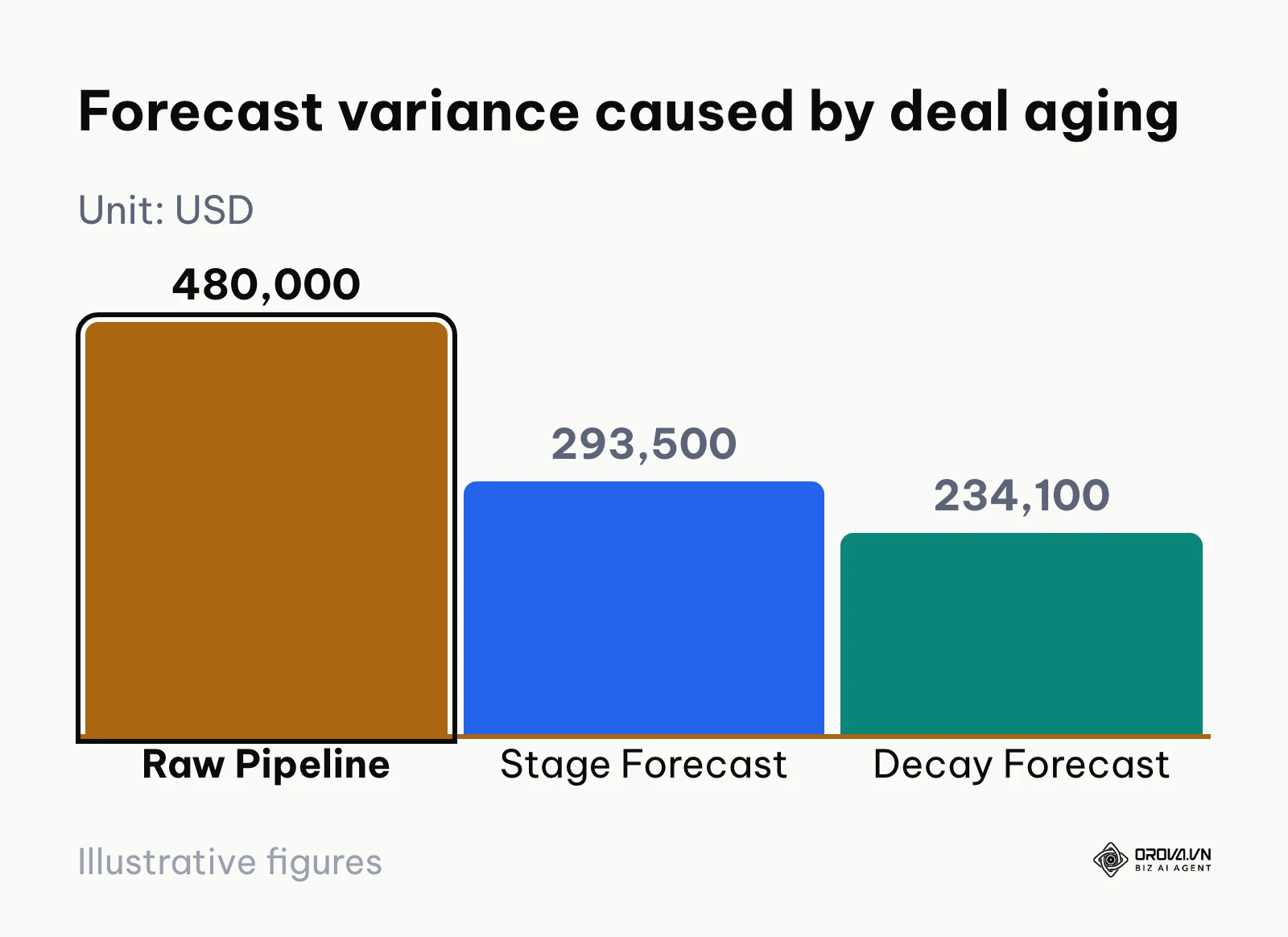
Total / Summary	480,000	—	—	—	—	234,100

Under a standard, unadjusted stage probability calculation, this five-deal pipeline would be reported to executive leadership as 293,500 dollars (25,000 + 90,000 + 4,500 + 24,000 + 150,000). Applying an objective aging decay adjustment reveals that the true mathematical expected value is only 234,100 dollars, exposing a 59,400 dollar deficit caused entirely by stalled opportunities in Beta Inc and Delta Tech.

Sales cycle length forecasting is fundamentally superior at surfacing deal stagnation, whereas stage probability requires explicit mathematical decay adjustments to avoid presenting dangerously inflated numbers.

Implementation and CRM data requirements: Stage probability vs sales cycle length

Every forecasting model demands a specific level of underlying data hygiene. Organizations frequently fail when attempting advanced forecasting techniques because their CRM data architecture cannot support the mathematical prerequisites of the model.

Stage probability forecasting requires minimal historical data to implement initially. A sales leader can review the past 90 days of closed deals, estimate aggregate conversion rates across 4 to 6 stages, and configure fixed percentages in their CRM within a single morning. As long as sales representatives move deals across stages with reasonable consistency, the system generates continuous forecasts immediately. Maintaining high crm data quality is still necessary, but the barrier to entry is exceptionally low.

In contrast, sales cycle length forecasting requires deep, historically clean time-series data. To calculate a valid sales velocity projection, a company must possess:

1. Accurate, tamper-free creation dates for opportunities across at least two full sales cycle iterations.
2. Segmented cycle benchmarks categorized by lead source, deal size tiers, and target customer segments.
3. Clean stage-by-stage timestamp logs that record the exact duration deals spend in each intermediate phase.

If a company sells to both mid-market companies (20,000 dollars ACV, 45-day cycle) and enterprise conglomerates (150,000 dollars ACV, 180-day cycle), blending them into a single aggregate sales cycle duration corrupts the entire forecast calculation. For organizations with less than a year of operational CRM history, sales cycle length forecasting generates chaotic projections due to statistical noise and inadequate sample sizes.

Worked example:

• Context: A seed-stage B2B cybersecurity startup with two account executives and 4 months of CRM activity.
• Steps taken: The founder attempted to build an automated sales velocity model in a spreadsheet, projecting revenue based on an assumed 35-day sales cycle.
• Snag encountered & fix: Several deals closed in 12 days through personal networks, while several inbound pilot projects stalled at 70 days. The small sample size skewed the mathematical average, causing the model to forecast that three complex enterprise pilots would close simultaneously in the middle of month five. The founder abandoned the cycle duration model and established five basic pipeline stages with conservative milestone probabilities (10%, 25%, 50%, 75%).
• Visible operational result: The monthly pipeline forecast variance dropped from 48% to 14%, stabilizing cash flow projections for the founding team.

Stage probability is significantly easier and faster to implement for young or growing teams, while sales cycle forecasting requires mature data infrastructure and high transaction volumes to yield reliable results.

Tired of pipeline forecasts distorted by stale opportunities? Orova CRM features customizable drag-and-drop pipelines, automated stage-based revenue weighting reports, and an automatic deal recall engine that returns neglected leads to the unassigned pool based on stage-specific minute timeouts.

Managing rep subjectivity and stage exit criteria: Stage probability vs sales cycle length

The Achilles' heel of milestone-based forecasting has always been salesperson sentimentality, commonly referred to in sales management as "happy ears." When an account executive has an engaging conversation with a prospect, they instinctively advance the opportunity to "Negotiation" in the CRM to demonstrate activity and optimism, artificially spiking the weighted forecast.

Sales cycle length forecasting bypasses rep psychology entirely. The calendar does not care how enthusiastic the sales rep felt during Tuesday's meeting; if 60 days have passed on a deal that historically takes 30 days to close, the time-based algorithm deprioritizes the deal's near-term revenue contribution.

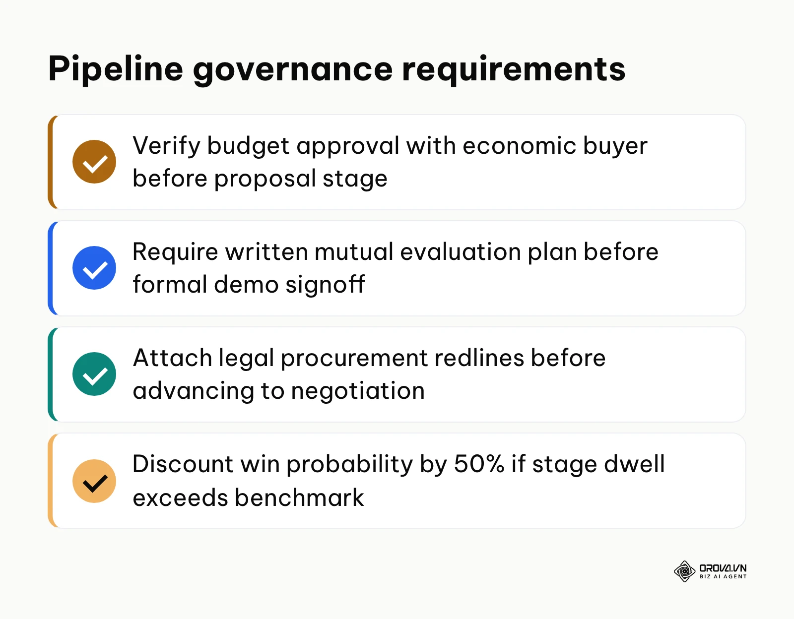
However, stage probability forecasting can be completely insulated against rep subjectivity by establishing verifiable pipeline stage exit criteria. A deal must never be advanced to a higher win probability based on rep intuition; promotion requires concrete documentary proof from the buyer. Effective crm sales pipeline management relies on enforcing objective gate checks at every phase of the funnel.

The checklist table below details five standard B2B sales pipeline stages alongside the mandatory actions and verifiable evidence required before a rep is permitted to advance an opportunity and increase its forecasted probability:

Pipeline Stage	Mandatory Rep Action	Verifiable Evidence Required	Assigned Probability
1. Discovery	Conduct structured problem exploration and qualify budget parameters	Signed discovery summary or mutual pain statement confirmed via email by prospect	10%
2. Solution Demo	Present tailored software architecture addressing identified pain points	Written mutual evaluation plan with confirmed test criteria and target completion date	25%
3. Proposal Review	Deliver customized commercial pricing, implementation scope, and SLA terms	Written confirmation from economic buyer that budget is allocated for the proposed scope	50%
4. Negotiation	Resolve technical objections, legal redlines, and information security terms	Redlined master services agreement (MSA) received directly from legal or procurement	75%
5. Closed Won	Execute final commercial agreement and process billing documentation	Countersigned agreement and formal client purchase order (PO) uploaded to CRM	100%

Enforcing these binary exit gates transforms stage probability from an exercise in emotional guessing into a disciplined governance mechanism. If a rep cannot attach the mutual evaluation plan, the deal remains locked at 10% probability, preserving forecast integrity.

Sales cycle length forecasting naturally eliminates rep bias through objective calendar data, but stage probability forecasting achieves equal or superior objectivity when reinforced with mandatory, verifiable stage exit criteria.

Pipeline coverage and quota attainment: Stage probability vs sales cycle length

Forecasting revenue is only half of the sales leadership equation; the other half is determining whether your open pipeline provides sufficient coverage to hit periodic targets. An executive does not merely want to know how much cash is projected to arrive; they need to know if the team must immediately generate additional pipeline to prevent a shortfall two quarters down the road.

Pipeline coverage ratio measures the total qualified pipeline value relative to the remaining quota for a given period:

$$\text{Pipeline Coverage Ratio} = \frac{\text{Qualified Pipeline Value}}{\text{Remaining Quota Target}}$$

Data from the Sales Development Benchmark Report released by TOPO in 2023 established that maintaining a 3.5x to 4.0x qualified pipeline coverage ratio remains the standard safety threshold for B2B teams managing 60-to-90-day deal velocities. If a department carries a quarterly quota of 500,000 dollars, it must maintain between 1,750,000 and 2,000,000 dollars in active, qualified pipeline at the start of the quarter to reliably hit quota.

Stage probability forecasting interacts directly with quota attainment metrics by translating gross coverage into "weighted coverage." While a team might possess a comfortable 4.0x gross pipeline coverage ratio, calculating the stage-weighted expected value might reveal only 0.85x quota coverage, warning the vice president of sales that too many deals are clustered in early, low-probability stages. Effective sales pipeline management requires balancing both top-of-funnel volume and late-stage progression.

Sales cycle length forecasting views coverage through the lens of timing windows. If a team has 4.0x coverage, but 70% of those opportunities are mathematically projected to close outside the current quarter based on historical velocity, the apparent coverage is an illusion.

Worked example:

• Context: A regional B2B telecom provider with a 1,200,000 dollar third-quarter revenue quota and 12 field sales representatives.
• Steps taken: The vice president of sales reviewed the gross pipeline, which stood at 4,800,000 dollars (a healthy 4.0x coverage ratio). Next, the VP ran both a stage-weighted calculation and a cycle-duration filter.
• Snag encountered & fix: The stage-weighted model projected 1,150,000 dollars in closed business (96% quota attainment). However, the cycle-length model flagged that 1,800,000 dollars of the pipeline had entered the funnel within the last 15 days, meaning their historical 75-day sales cycle would push their close dates into the fourth quarter. The VP immediately mobilized a blitz campaign targeting late-stage stalled proposals and accelerated contracting timelines with existing pipeline accounts.
• Visible operational result: The team secured 1,215,000 dollars before the end of September, hitting 101% of their quarterly target by prioritizing deal acceleration over top-of-funnel accumulation.

Stage probability forecasting is better for evaluating whether pipeline maturity matches revenue targets, while sales cycle length forecasting is essential for verifying whether that revenue will land inside the current calendar quarter.

When to choose stage probability forecasting

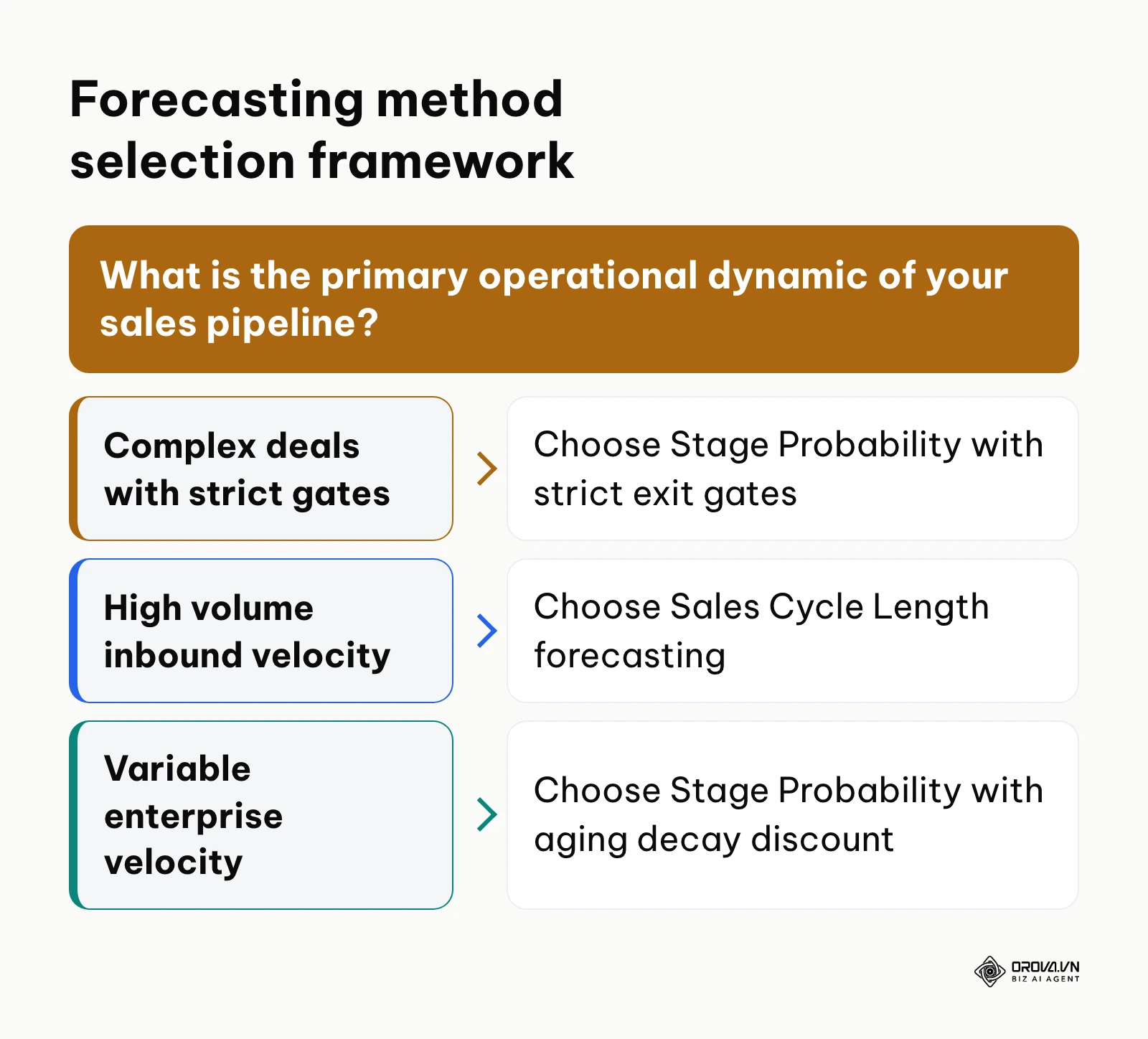
Stage probability forecasting remains the gold standard for organizations operating complex sales motions with clearly delineated milestones. You should implement stage probability forecasting when your business matches the following operational conditions:

1. Enterprise and Custom Solution Sales: Your average deal size exceeds 25,000 dollars, involving multiple buyer stakeholders, customized scopes of work, and prolonged procurement reviews. In enterprise deals, milestone verification (such as passing a security review) represents a far more reliable indicator of closing than how many days the deal has been open.
2. Strict Pipeline Governance Capabilities: Your organization has the operational discipline to define and enforce binary exit criteria. When sales reps understand that opportunities cannot advance without verifiable documentary proof, stage probability yields exceptionally dependable forecasts.
3. Variable Contract Values: Your pipeline contains deals ranging from 10,000 to 250,000 dollars. Applying a uniform time-decay model to deals of vastly different sizes leads to distorted averages, whereas weighting each specific deal by its verified milestone position preserves deal-level context.
4. Sales Rep Coaching and Accountability Focus: Stage-based forecasting allows frontline managers to pinpoint exact friction points in the funnel during one-on-one deal reviews. If deals consistently stall between "Solution Demo" and "Proposal Review," management can implement targeted training on objection handling or commercial packaging.

When to choose sales cycle length forecasting

Sales cycle length forecasting is the superior methodology for organizations prioritizing velocity, volume, and statistical objectivity over individual deal mechanics. Before selecting this approach, review how your pipeline parameters compare across these core operational criteria:

Evaluation Parameter	Stage Probability Forecasting	Sales Cycle Length Forecasting	Recommended Selection Rule
Average Deal Size	> 25,000 dollars (multi-stakeholder B2B)	< 10,000 dollars (standardized transaction)	Stage Probability for Enterprise; Cycle for Velocity
Monthly Deal Volume	< 20 opportunities per rep	> 40 opportunities per rep	High volume favors law of large numbers in Cycle
Pipeline Stage Rigor	Verifiable buyer exit documents	Unstructured or rapid progression	Strict stage gates required for Stage Probability
Historical Data Log	60 to 90 days conversion history	12+ months clean duration logs	Young startups must start with Stage Probability
Rep Behavioral Bias	High optimism bias ("happy ears")	Objective automated timestamps	Cycle length removes rep sentimentality

You should implement sales cycle length forecasting under the following circumstances:

1. High-Velocity Inbound or Transactional B2B: Your sales cycle averages between 14 and 45 days, deal sizes are relatively uniform (such as tiered SaaS subscriptions or standardized commercial services), and transaction volume exceeds 50 closed deals per month. Under these conditions, the law of large numbers smooths out individual anomalies.
2. Limited Administrative Capacity: Your sales team spends minimal time manually logging detailed qualitative notes or collecting formal buyer confirmation documents. Cycle length relies on automated system timestamps (creation date, stage change date), eliminating administrative burden for reps.
3. Mature Historical CRM Datasets: Your business has operated for at least 12 to 24 months with clean, continuous CRM tracking, allowing you to establish accurate duration baselines across different lead sources, product tiers, and sales reps.
4. Severe Past Forecasting Inaccuracies Caused by Rep Optimism: If your executive team has experienced recurring quarterly revenue misses due to sales reps hoarding stagnant opportunities and claiming they are "about to close," adopting an automated time-in-stage model immediately cleanses the pipeline of wishful thinking.

Build predictable revenue projections in minutes without manual spreadsheet gymnastics. Configure custom pipeline stages, track quota attainment across days, weeks, months, or quarters, and manage departmental visibility in Orova CRM. Free until July 7, 2027 with full feature access.

Can you combine both forecasting methods?

High-performing revenue operations teams rarely rely on a single forecasting technique in isolation. Instead of treating stage probability and sales cycle length as mutually exclusive alternatives, modern revenue teams combine them into a hybrid dynamic forecasting engine.

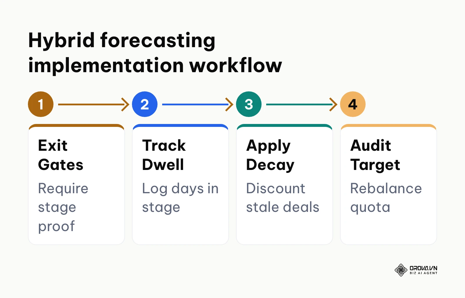
In a hybrid model, opportunity stage probability serves as the foundational revenue anchor, while sales cycle velocity acts as a dynamic discount modifier. When a deal reaches the proposal stage, it is assigned a baseline 50% win probability. If the deal progresses within the historical 30-day benchmark for that stage, it retains its full 50% weighting. However, if the deal remains in that stage on Day 45 without moving to contract negotiation, an automated system script applies a 50% aging decay penalty, reducing its operational probability to 25%. If it reaches Day 60 without verifiable activity, its forecasted value drops to 10% or is automatically removed from the primary forecast report.

Transitioning from a basic stage-probability model to a hybrid framework involves four structured operational milestones:

Implementation Phase	Operational Milestone	Technical CRM Mechanism	Audit Frequency
Phase 1: Governance	Lock Stage Exit Gates	Mandatory document attachment fields	Weekly deal reviews
Phase 2: Benchmarking	Calculate Dwell Baselines	Historical time-in-stage duration logs	Quarterly calibration
Phase 3: Automation	Program Dynamic Aging Formulas	Automated decay modifiers (50% and 80%)	Continuous reporting
Phase 4: Hygiene	Enforce Reallocation Triggers	Automated unassigned recall rules	Daily pipeline sweeps

Executing these four phases ensures that pipeline progression remains verifiable while deal aging automatically deflates phantom forecast numbers.

The primary risk in executing a hybrid model is over-engineering reporting complexity. If sales managers must spend hours recalculating decaying percentages by hand across disparate spreadsheets, adherence will collapse within weeks.

This is precisely where the architecture of Orova CRM provides structural operational value. Orova CRM allows sales leaders to establish customized, drag-and-drop pipelines with distinct stages, while generating automated overview reports that calculate stage-weighted revenue projections strictly through mathematical stage conversion rules rather than opaque AI estimations. Furthermore, Orova CRM includes an automated deal recall mechanism that actively scans the pipeline and retrieves neglected customer records back to the shared pool based on customizable minute-level timeouts per stage. Combined with quota tracking capabilities that measure performance by department or individual across daily, weekly, monthly, quarterly, or yearly cycles, teams maintain pristine pipeline hygiene without manual spreadsheet overhead.

Future trends in sales pipeline forecasting: author's perspective

Looking at the trajectory of revenue operations as of 2026, the traditional distinction between milestone tracking and time tracking is dissolving into unified behavioral telemetry. Below are three distinct structural shifts I expect will redefine sales pipeline forecasting over the next two to three years.

First, I believe static, unadjusted stage probability percentages will disappear entirely from modern CRM architectures by 2028. Today, revenue leaders are already frustrated by the sheer volume of "ghost pipeline" distorting their quarterly forecasts, and finance executives are demanding that pipeline value be discounted continuously based on real-time deal aging. In my view, within three years, every professional CRM platform will automatically incorporate native dwell-time decay into its standard weighted revenue calculations, rendering static 50% or 75% multipliers obsolete. Sales leaders should prepare today by auditing historical stage dwell times and establishing benchmark velocity baselines across their product lines.

Second, I expect that artificial intelligence will prove most valuable in sales forecasting not as an autonomous revenue predictor, but as an aggressive pipeline auditor. The current wave of generative hype has led many vendors to promise black-box predictive models that guess deal outcomes using ambiguous sentiment analysis. However, enterprise sales leaders are quickly discovering that these algorithms fail whenever market conditions shift or buyer procurement structures change. Instead, I foresee AI agents focusing on continuous pipeline hygiene: automatically detecting inconsistencies, verifying documentary evidence against exit criteria, and flagging discrepancies between rep notes and buyer communications. If enterprise software platforms fail to make AI outputs transparent and auditable, sales organizations will reject automated forecasting tools in favor of simple, auditable mathematical rules.

Third, I anticipate a major convergence between pipeline progression and actual cash collection milestones. In today's landscape, most CRMs treat the pipeline as concluded the moment a deal reaches "Closed Won," leaving accounts receivable and invoice payment tracking to separate accounting applications. Over the coming years, B2B forecasting models will expand their definitions to include post-signature cash realization, recognizing that a closed contract that takes 90 days to settle payment represents a velocity drag on operating cash flow. Revenue teams should begin aligning sales pipeline reporting directly with billing terms and milestone collection schedules now.

Frequently asked questions about sales pipeline forecasting methods

How do you adjust a deal's win probability when it lingers in a stage twice as long as the average sales cycle?

When an opportunity dwells in an intermediate pipeline stage longer than twice the historical average duration, best practice dictates reducing its assigned win probability by at least 50% to 80%. If the benchmark dwell time for a negotiation stage is 20 days and an active deal has sat untouched for 45 days, its base 75% probability should be manually or automatically discounted to between 15% and 37.5%. If no verifiable customer engagement occurs within three times the benchmark duration, the opportunity should be marked as closed-lost or returned to a marketing nurture sequence.

What is a safe pipeline coverage ratio for B2B companies with 30-to-90-day sales cycles?

For B2B organizations operating within a 30-to-90-day sales cycle window, a safe qualified pipeline coverage ratio is between 3.5x and 4.0x of the periodic quota. A 4.0x coverage ratio provides adequate buffer against inevitable deal slippage, procurement delays, and unexpected competitive losses. Teams with highly transactional, shorter cycles (under 30 days) can operate safely with 2.5x to 3.0x coverage, while enterprise organizations managing 6-month cycles often require 4.5x to 5.0x coverage to ensure quota attainment.

How do you eliminate sales rep over-optimism when categorizing deals into Commit and Best Case?

Eliminating sales rep bias requires replacing subjective emotional classifications with verifiable buyer evidence. Reps must be prohibited from placing deals into "Commit" categories unless specific, documented buyer milestones have been completed and uploaded to the CRM, such as a formal confirmation of budget allocation from the economic buyer and a redlined contract undergoing final procurement review. If a deal only possesses verbal interest or unconfirmed timelines, it must remain in the "Best Case" or "Pipeline" category regardless of the rep's reported confidence.

What role does artificial intelligence play in sales pipeline forecasting methods?

Artificial intelligence enhances sales pipeline forecasting primarily by automating pipeline hygiene and identifying operational anomalies rather than attempting to guess future revenue out of thin air. Modern AI tools analyze historical stage conversion trends, flag stagnant deals that deviate from established velocity norms, and audit communications to ensure deals are not prematurely advanced without required documentation. However, core revenue forecasting calculations should remain grounded in transparent mathematical formulas—such as stage probability and historical velocity decay—so leadership can trace every projected dollar back to auditable metrics.

Can a small business with under five sales reps use sales cycle length forecasting?

A small business with fewer than five sales representatives can use sales cycle length forecasting only if it processes a high volume of standardized, transactional deals (at least 30 to 40 closed transactions per month). If the business closes only 3 to 5 custom enterprise contracts per quarter, sample size limitations will make sales cycle averages statistically unreliable. In low-volume environments, small businesses should rely on stage probability forecasting reinforced by rigid, documented exit criteria.

Where should you start?

Improving your revenue predictability does not require an immediate, multi-month overhaul of your entire sales technology stack. Your immediate priority should be executing a single high-impact operational step tailored to your current CRM situation.

If your CRM data is currently cluttered with stale opportunities and zero stage discipline, your immediate task this afternoon is to conduct an aggressive pipeline audit. Pull a report of all open deals across every pipeline stage and filter by days since last customer touchpoint. Immediately mark every deal that has sat inactive for more than twice your average sales cycle as closed-lost or move it into an unassigned recycling queue. Purging this phantom pipeline will instantly reveal your true revenue baseline.

If your sales team has grown to several account executives but consistently misses quarterly revenue forecasts due to optimistic projections, your immediate step is to define and publish binary exit criteria for your two most critical pipeline stages (typically Solution Demo and Proposal Review). Gather your sales managers, draft a mandatory document checklist for each of those two stages, and configure your CRM so reps cannot advance opportunities without attaching verifiable proof of customer commitment.

If your organization already possesses clean stage discipline and predictable deal flow, your focus should shift to building a dynamic decay model. Spend an afternoon calculating your historical average dwell times for each intermediate funnel stage over the past two quarters, and introduce an aging penalty rule into your executive reporting spreadsheet to discount deals that linger past their expected close dates.

By matching your organizational maturity with the appropriate operational mechanics, you can transform your sales pipeline forecasting methods from subjective guesswork into a reliable engine for sustainable business growth.